Merge sort is one of the basic computer science algorithms, formulated back in 1945 by the great mathematician John von Neumann. While participating in the Manhattan Project, Neumann was faced with the need to efficiently process huge amounts of data. The method he developed used the principle of "divide and conquer", which significantly reduced the time required for work.
Principle and use of the algorithm
The merge sort method is used in problems of sorting structures that have ordered access to elements, such as arrays, lists, streams.
During processing, the initial data block is split into small components, up to one element, which in fact is already a sorted list. Then it is reassembled in the correct order.
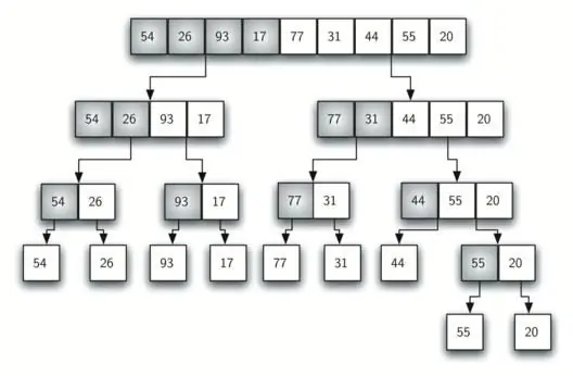
Sorting an array of a certain length requires an additional memory area of the same size, in which the sorted array is collected in parts.
The method can be used to order any comparable data type, such as numbers or strings.
Merge sortedplots
To understand the algorithm, let's start its analysis from the end - from the mechanism of merging sorted blocks.
Let's imagine that we have two arrays of numbers sorted in any way that need to be combined with each other so that the sorting is not broken. For simplicity, we will sort the numbers in ascending order.
Elementary example: both arrays consist of one element each.
int arr1={31}; int arr2={18};
To merge them, you need to take the zero element of the first array (don't forget that numbering starts from zero) and the zero element of the second array. These are, respectively, 31 and 18. According to the sorting condition, the number 18 should come first, since it is less. Just put the numbers in the correct order:
int result={18, 31};
Let's look at a more complicated example, where each array consists of several elements:
int arr1={2, 17, 19, 45}; int arr2={5, 6, 21, 30};
The merge algorithm will consist of sequentially comparing smaller elements and placing them in the resulting array in the correct order. To keep track of the current indices, let's introduce two variables - index1 and index2. Initially, we set them to zero, since the arrays are sorted, and the smallest elements are at the beginning.
int index1=0; int index2=0;
Let's write the whole merging process step by step:
- Take the element with index1 from the array arr1, and the element with index2 from the array arr2.
- Compare, select the smallest of them and put inresulting array.
- Increment the current index of the smaller element by 1.
- Continue from the first step.
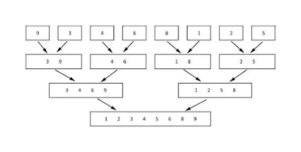
On the first orbit, the situation will look like this:
index1=0; index2=0; arr1[0]=2; arr2[0]=5; arr1[0] < arr2[0]; index1++; result[0]=arr1[0]; // result=[2]
On the second turn:
index1=1; index2=0; arr1[1]=17; arr2[0]=5; arr1[1] > arr2[0]; index2++; result[1]=arr2[0]; // result=[2, 5]
Third:
index1=1; index2=1; arr1[1]=17; arr2[1]=6; arr1[1] > arr2[1]; index2++; result[2]=arr2[1]; // result=[2, 5, 6]
And so on, until the result is a completely sorted array: {2, 5, 6, 17, 21, 19, 30, 45}.
Certain difficulties can arise if arrays with different lengths are merged. What if one of the current indexes has reached the last element, and there are still members left in the second array?
int arr1={1, 4}; int arr2={2, 5, 6, 7, 9}; // 1 step index1=0, index2=0; 1 2 result={1, 2}; // 3 step index1=1, index2=1; 4 < 5 result={1, 2, 4}; //4 step index1=2, index2=1 ??
The index1 variable has reached the value 2, but the arr1 array does not have an element with that index. Everything is simple here: just transfer the remaining elements of the second array to the resulting array, preserving their order.
result={1, 2, 4, 5, 6, 7, 9};
This situation indicates to us the needmatch the current check index with the length of the array being merged.
Merge scheme for ordered sequences (A and B) of different lengths:
- If the length of both sequences is greater than 0, compare A[0] and B[0] and move the smaller one to the buffer.
- If the length of one of the sequences is 0, take the remaining elements of the second sequence and, without changing their order, move to the end of the buffer.
Implementation of the second stage
An example of joining two sorted arrays in Java is given below.
int a1=new int {21, 23, 24, 40, 75, 76, 78, 77, 900, 2100, 2200, 2300, 2400, 2500}; int a2=new int {10, 11, 41, 50, 65, 86, 98, 101, 190, 1100, 1200, 3000, 5000}; int a3=new int[a1.length + a2.length]; int i=0, j=0; for (int k=0; k a1.length-1) { int a=a2[j]; a3[k]=a; j++; } else if (j > a2.length-1) { int a=a1; a3[k]=a; i++; } else if (a1 < a2[j]) { int a=a1; a3[k]=a; i++; } else { int b=a2[j]; a3[k]=b; j++; } }
Here:
- a1 and a2 are the original sorted arrays to be merged;
- a3 - final array;
- i and j are indexes of current elements for arrays a1 and a2.
The first and second if conditions ensure that the indexes do not go beyond the size of the array. The third and fourth condition blocks, respectively, are moved to the resulting array of the smaller element.
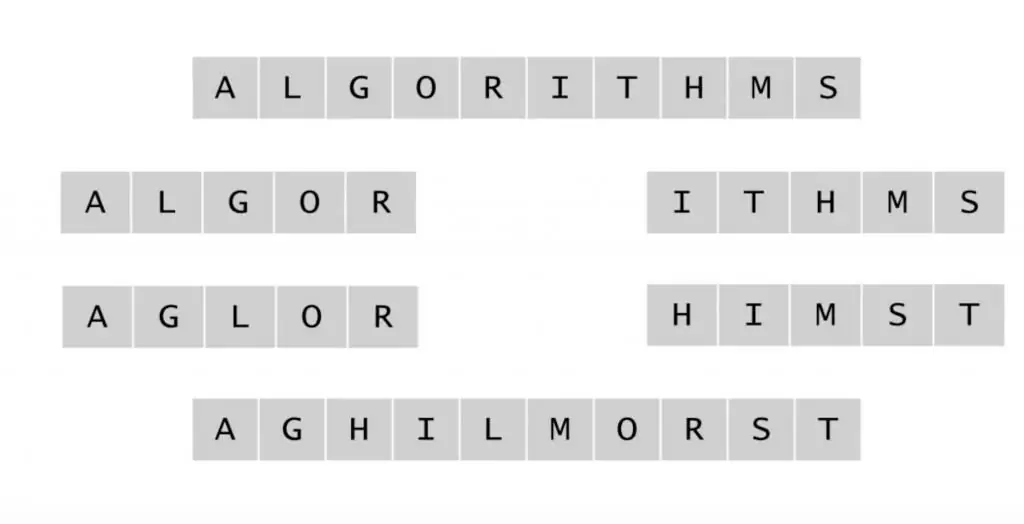
Divide and Conquer
So, we have learned to merge the sortedcollections of values. It can be said that the second part of the merge sort algorithm - the merge itself - has already been sorted.
However, you still need to understand how to get from the original unsorted array of numbers to several sorted ones that can be merged.
Let's consider the first stage of the algorithm and learn how to separate arrays.
This is not difficult - the original list of values is divided in half, then each part is also bifurcated, and so on until very small blocks are obtained.
The length of such minimal elements can be equal to one, that is, they can themselves be a sorted array, but this is not a necessary condition. The size of the block is determined in advance, and any suitable sorting algorithm that works efficiently with arrays of small sizes (for example, quicksort or insertion sort) can be used to order it.
It looks like this.
// original array {34, 95, 10, 2, 102, 70}; // first split {34, 95, 10} and {2, 102, 70}; // second split {34} and {95, 10} and {2} and {102, 70}
The resulting blocks, consisting of 1-2 elements, are very easy to arrange.
After that, you need to merge the already sorted small arrays in pairs, preserving the order of the members, which we have already learned to do.
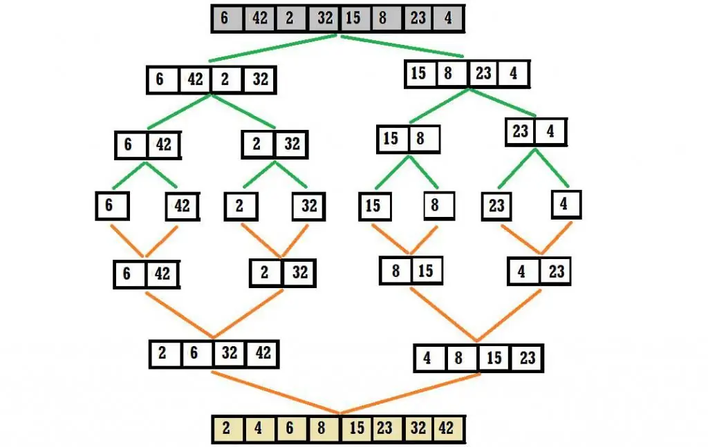
Implementation of the first stage
Recursive partitioning of an array is shown below.
void mergeSort(T a, long start, long finish) { long split; if(start < finish) { split=(start + finish)/2; mergeSort(a, start, split); mergeSort(a, split+1, finish); merge(a, start, split, finish); } }
What happens in this code:
-
The mergeSort function gets the initial array
a
and the left and right borders of the region to be sorted (indices start and
- finish).
-
If the length of this section is greater than one (
start < finish
), then it is split into two parts (by index
- split), and each one is recursively sorted.
-
The initial index of the plot and the index
split
are passed to the recursive function call for the left side. For the right one, respectively, the beginning will be
- (split + 1), and the end will be the last index of the original section.
-
Function
merge
gets two ordered sequences (
a[start]…a[split]
and
- a[split +1]…a[finish]) and merges them in sort order.
The mechanics of the merge function are discussed above.
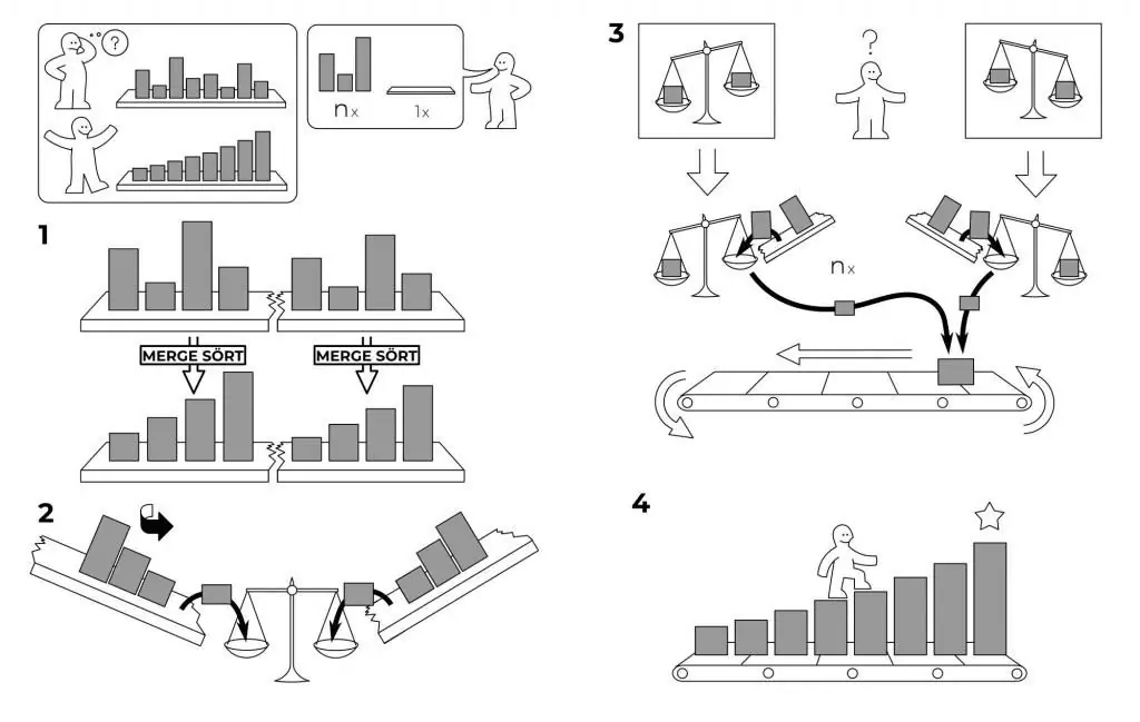
General scheme of the algorithm
The merge sort array method consists of two large steps:
- Split the unsorted original array into small pieces.
- Collect them in pairs, following the sorting rule.
A large and complex task is broken down into many simple ones, which are sequentially solved, leading to the desired result.
Method evaluation
The time complexity of merge sort is determined by the height of the split treealgorithm and is equal to the number of elements in the array (n) times its logarithm (log n). Such an estimate is called logarithmic.
This is both an advantage and a disadvantage of the method. Its running time does not change even in the worst case, when the original array is sorted in reverse order. However, when processing completely sorted data, the algorithm does not provide a time gain.
It is also important to note the memory cost of the merge sort method. They are equal to the size of the original collection. In this additionally allocated area, a sorted array is assembled from the pieces.
Implementation of the algorithm
Pascal merge sort is shown below.
Procedure MergeSort(name: string; var f: text); Var a1, a2, s, i, j, kol, tmp: integer; f1, f2: text; b: boolean Begincol:=0; Assign(f, name); reset(f); While not EOF(f) do begin read(f, a1); inc(col); end; close(f); Assign(f1, '{name of 1st auxiliary file}'); Assign(f2, '{name of 2nd auxiliary file}'); s:=1; While (s<kol) do begin Reset(f); rewrite(f1); rewrite(f2); For i:=1 to kol div 2 do begin Read(f, a1); Write(f1, a1, ' '); end; If (kol div 2) mod s0 then begin tmp:=kol div 2; While tmp mod s0 do begin Read(f, a1); Write(f1, a1, ' '); inc(tmp); end; end; While not EOF(f) do begin Read(f, a2); Write(f2, a2, ' '); end; close(f); close(f1); close(f2); rewrite(f); reset(f1); reset(f2); Read(f1, a1); Read(f2, a2); While (not EOF(f1)) and (not EOF(f2)) do begin i:=0; j:=0; b:=true; While (b) and (not EOF(f1)) and (not EOF(f2)) do begin If (a1<a2) then beginWrite(f, a1, ' '); Read(f1, a1); inc(i); End else begin Write(f, a2, ' '); Read(f2, a2); inc(j); end; If (i=s) or (j=s) then b:=false; end; If not b then begin While (i<s) and (not EOF(f1)) do begin Write(f, a1, ' '); Read(f1, a1); inc(i); end; While (j<s) and (not EOF(f2)) do begin Write(f, a2, ' '); Read(f2, a2); inc(j); end; end; end; While not EOF(f1) do begin tmp:=a1; Read(f1, a1); If not EOF(f1) then Write(f, tmp, ' ') else Write(f, tmp); end; While not EOF(f2) do begin tmp:=a2; Read(f2, a2); If not EOF(f2) then Write(f, tmp, ' ') else Write(f, tmp); end; close(f); close(f1); close(f2); s:=s2; end; Erase(f1); Erase(f2); End;
Visually, the operation of the algorithm looks like this (top - unordered sequence, bottom - ordered).

External data sorting
Very often there is a need to sort some data located in the external memory of the computer. In some cases, they are of impressive size and cannot be placed in RAM to facilitate access to them. For such cases, external sorting methods are used.
The need to access external media degrades processing time efficiency.
The complexity of the work is that the algorithm can only access one element of the data stream at a time. And in this case, one of the best results is shown by the merge sort method, which can compare the elements of two files sequentially one after the other.
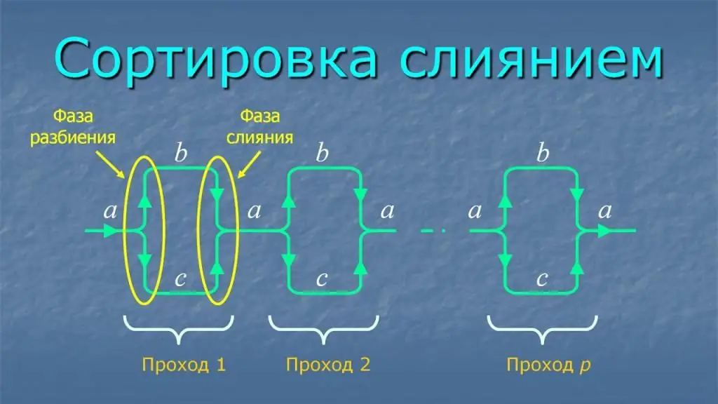
Reading data fromexternal source, their processing and writing to the final file are carried out in ordered blocks (series). According to the way of working with the size of ordered series, there are two types of sorting: simple and natural merging.
Simple merge
With a simple merge, the series length is fixed.
Thus, in the original unsorted file, all series consist of one element. After the first step, the size increases to two. Next - 4, 8, 16 and so on.
It works like this:
- The source file (f) is divided into two auxiliary ones - f1, f2.
- They are again merged into one file (f), but at the same time all elements are compared in pairs and form pairs. The series size at this step becomes two.
- Step 1 is repeated.
- Step 2 is repeated, but the already ordered 2s are merged to form sorted 4s.
- The loop continues, increasing the series on each iteration, until the entire file is sorted.
How do you know that the outer sorting with a simple merge is complete?
- new series length (after merging) not less than the total number of elements;
- only one episode left;
- Auxiliary file f2 was left empty.
The disadvantages of a simple merge are: since the run length is fixed on each merge pass, partially ordered data will take as long to process as completely random data.
Natural fusion
This method does not limit the lengthseries, but chooses the maximum possible.
Sorting algorithm:
- Reading the initial sequence from file f. The first received element is written to the file f1.
- If the next entry satisfies the sorting condition, it is written there, if not, then to the second auxiliary file f2.
- In this way, all records of the source file are distributed, and an ordered sequence is formed in f1, which determines the current size of the series.
- Files f1 and f2 are merged.
- The cycle repeats.
Due to the non-fixed size of the series, it is necessary to mark the end of the sequence with a special character. Therefore, when merging, the number of comparisons increases. In addition, the size of one of the auxiliary files may be close to the size of the original.
On average, natural merge is more efficient than simple merge with external sort.
Features of the algorithm
When comparing two identical values, the method preserves their original order, that is, it is stable.
The sorting process can be very successfully split into multiple threads.
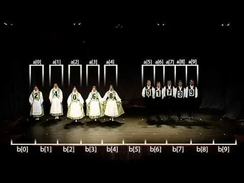
The video clearly demonstrates the operation of the merge sort algorithm.


